import numpy as np
import mplcyberpunk

import matplotlib.pyplot as plt
from scipy.stats import norm
plt.style.use("cyberpunk")Fourier Series
Any function \(f(t)\) that is periodic with period \(T\) can be decomposed as a sum of sines and cosines: \[
f(t) = a_0 + \sum_{n=1}^{\infty} a_n\cos(\omega_nt) + b_n\sin(\omega_nt)
\] where \(\omega_n = \frac{2\pi n}{T}\) and the coefficients \(a_n\) and \(b_n\) are given by: \[
a_n = \frac{2}{T}\int_{0}^{T} f(t)\cos(\omega_nt)dt= \frac{1}{||\cos(\omega_nt)||^2}\langle f(t), \cos(\omega_nt)\rangle
\] \[
b_n = \frac{2}{T}\int_{0}^{T} f(t)\sin(\omega_nt)dt= \frac{1}{||\sin(\omega_nt)||^2}\langle f(t), \sin(\omega_nt)\rangle
\]
The coefficients \(a_n\) and \(b_n\) are the Fourier series coefficients of the function \(f(t)\). The coefficients are inner products of Hilbert spaces. The inner product of two functions \(f(t)\) and \(g(t)\) is defined as: \[
\langle f, g \rangle = \int_{0}^{T} f(t)g(t)dt
\]
Here’s a note on dot product in vector space, which measures how closely two vectors are aligned. The dot product of two vectors \(a\) and \(b\) is defined as: \[ \langle a, b\rangle = ||a||\cdot||b||\cos(\theta) \] If they are perfectly aligned, the angle \(\theta = 0\) and the dot product is maximized due to \(\cos(0) = 1\). If they are orthogonal, the angle \(\theta = \frac{\pi}{2}\) and the dot product is zero due to \(\cos(\frac{\pi}{2}) = 0\). In Hilbert space, the inner product generalizes the dot product to functions, but they share the same idea of measuring how closely two functions are aligned.
# Define the functions
x = np.linspace(-10, 10, 500)  # A range of x values

# Function f: Standard normal distribution (PDF)
f = norm.pdf(x, 0, 3)

# Function g: Cosine function
g = np.sin(x)

# Product of f and g
fg = f * g

fig, axs = plt.subplots(2, 2, figsize=(10, 8))

axs[0, 0].plot(x, f, color='blue')
axs[0, 0].set_title('Standard Normal Distribution (f)')
axs[0, 0].grid(True)

axs[0, 1].plot(x, g, color='green')
axs[0, 1].set_title('Sine Function (g)')
axs[0, 1].grid(True)

axs[1, 0].plot(x, fg, color='purple')
axs[1, 0].set_title('Product of f and g (f * g)')
axs[1, 0].grid(True)

axs[1, 1].plot(x, fg, color='orange')
axs[1, 1].fill_between(x, fg, color='orange', alpha=0.3)  # Shade under the curve
axs[1, 1].set_title('Shaded Area under f * g')
axs[1, 1].grid(True)

# Adjust layout and display the plot
plt.tight_layout()
mplcyberpunk.add_glow_effects()
plt.show()
But what are $ $ and $ $? They are the norms of \(\cos(\omega_nt)\) and \(\sin(\omega_nt)\), respectively. In linear algebra, we have discussed Gram-Schmidt process, which is a method to orthogonalize a set of vectors.
In finite dimension, the projection of vector \(\mathbf{v}\) onto \(\mathbf{u}\) is given by:
\[ \operatorname{proj}_{\mathbf{u}} \mathbf{v}=\left(\frac{\mathbf{v} \cdot \mathbf{u}}{\|\mathbf{u}\|^2}\right) \mathbf{u} \]
The scalar \(\frac{\mathbf{v} \cdot \mathbf{u}}{\|\mathbf{u}\|^2}\) tells us how much of \(\mathbf{u}\) is in \(\mathbf{v}\), adjusted for the length of \(\mathbf{u}\).
u = np.array([3, 1])
v = np.array([2, 3])

proj_scalar = np.dot(v, u) / np.dot(u, u)
proj_v_on_u = proj_scalar * u

ortho = v - proj_v_on_u

plt.figure(figsize=(8, 8))
ax = plt.gca()

plt.quiver(0, 0, u[0], u[1], angles='xy', scale_units='xy', scale=1, color='blue', label=r'$\mathbf{u}$')

plt.quiver(0, 0, v[0], v[1], angles='xy', scale_units='xy', scale=1, color='red', label=r'$\mathbf{v}$')

plt.quiver(0, 0, proj_v_on_u[0], proj_v_on_u[1], angles='xy', scale_units='xy', scale=1,
           color='green', label=r'$\operatorname{proj}_{\mathbf{u}} \mathbf{v}$')

plt.plot([proj_v_on_u[0], v[0]], [proj_v_on_u[1], v[1]], linestyle='--',
         label=r'$\mathbf{v} - \operatorname{proj}_{\mathbf{u}} \mathbf{v}$')

plt.plot([v[0], proj_v_on_u[0]], [v[1], proj_v_on_u[1]], linewidth=1)

max_val = max(np.max(np.abs(u)), np.max(np.abs(v))) + 1
plt.xlim(-1, max_val)
plt.ylim(-1, max_val)
plt.xlabel('X-axis')
plt.ylabel('Y-axis')
plt.title('Projection of $\mathbf{v}$ onto $\mathbf{u}$')
plt.legend()

plt.axis('equal')

plt.grid(True)
plt.show()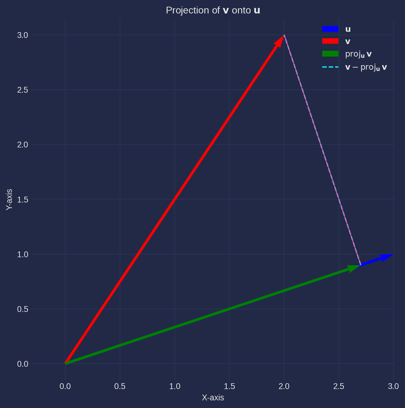
And you can prove that \[ \int_0^T \cos ^2\left(\omega_n t\right) d t=\frac{T}{2} \]
Substitute this into the integral:
\[ \int_0^T \cos ^2\left(\omega_n t\right) d t=\int_0^T \frac{1+\cos \left(2 \omega_n t\right)}{2} d t \]
Break the integral into two parts:
\[ \int_0^T \frac{1+\cos \left(2 \omega_n t\right)}{2} d t=\frac{1}{2} \int_0^T 1 d t+\frac{1}{2} \int_0^T \cos \left(2 \omega_n t\right) d \]
Evaluate the first integral:
\[ \frac{1}{2} \int_0^T 1 d t=\frac{1}{2} \times T=\frac{T}{2} \]
Evaluate the second integral:
\[ \int_0^T \cos \left(2 \omega_n t\right) d t \]
Since \(\cos \left(2 \omega_n t\right)\) is a periodic function with period \(\frac{\pi}{\omega_n}\), its integral over a zero:
\[ \int_0^T \cos \left(2 \omega_n t\right) d t=0 \]
Combine the results:
\[ \int_0^T \cos ^2\left(\omega_n t\right) d t=\frac{T}{2}+0=\frac{T}{2} \] And this is the reason we use \(T/2\) in the denominator of the Fourier series coefficients. The \(T/2\) term is the norm of \(\cos(\omega_nt)\) and \(\sin(\omega_nt)\), which is the length of the vector in Hilbert space. The \(T/2\) term is used to normalize the coefficients to make them unit vectors in Hilbert space.
Trignometric Orthogonality
But why using trigonometric functions? The simple reason is that trigonometric functions are orthogonal to each other, for instance \(\cos(\omega_nt)\) and \(\cos(\omega_mt)\) are orthogonal to each other if \(n \neq m\).
As a reminder, we all learn the product rule of sine and cosine in our high school: \[ \cos(a)\sin(b) = \frac{1}{2}[\sin(a+b) + \sin(a-b)] \] The inner product of \(\cos(\omega_nt)\) and \(\sin(\omega_mt)\) using product rule is: $$
\[\begin{aligned} \langle \cos(\omega_nt), \sin(\omega_mt) \rangle &= \int_{0}^{T} \cos(\omega_nt)\sin(\omega_mt)dt \\ &= \frac{1}{2}\int_{0}^{T} \sin(\omega_nt + \omega_mt) + \sin(\omega_nt - \omega_mt)dt \\ &= \frac{1}{2}\int_{0}^{T} \sin((\omega_n + \omega_m)t) + \sin((\omega_n - \omega_m)t)dt \\ &= \frac{1}{2}\left[\frac{-\cos((\omega_n + \omega_m)t)}{\omega_n + \omega_m} + \frac{-\cos((\omega_n - \omega_m)t)}{\omega_n - \omega_m}\right]_{0}^{T} \\ &= \frac{1}{2}\left[\frac{-\cos(2\pi(n+m))}{\omega_n + \omega_m} + \frac{-\cos(2\pi(n-m))}{\omega_n - \omega_m} - \frac{-\cos(0)}{\omega_n + \omega_m} - \frac{-\cos(0)}{\omega_n - \omega_m}\right] \\ &= \frac{1}{2}\left[\frac{-\cos(0)}{\omega_n + \omega_m} + \frac{-\cos(0)}{\omega_n - \omega_m} - \frac{-\cos(0)}{\omega_n + \omega_m} - \frac{-\cos(0)}{\omega_n - \omega_m}\right] \\ &= 0 \end{aligned}\]And this shows that \(\cos(\omega_nt)\) and \(\sin(\omega_mt)\) are orthogonal to each other. The same can be shown for \(\cos(\omega_nt)\) and \(\cos(\omega_mt)\) and \(\sin(\omega_nt)\) and \(\sin(\omega_mt)\) too.
Fourier Transform of a Symmetric Function
import numpy as np
import matplotlib.pyplot as plt

dx = 0.01
x = np.pi * np.arange(-1, 1, dx)
n = 10  # Number of terms
f = -x ** 10 # Target function

a0 = np.sum(f) * dx

a = np.zeros(n)
b = np.zeros(n)

fourier_series = a0 / 2

plt.figure(figsize=(10, 6))

plt.plot(x, f, label='Target function $f(x) = x^2$', color='blue')

for i in range(n):
    a[i] = np.sum(f * np.cos((i + 1) * x)) * dx
    b[i] = np.sum(f * np.sin((i + 1) * x)) * dx
    fourier_series += a[i] * np.cos((i + 1) * x) + b[i] * np.sin((i + 1) * x)

    plt.plot(x, fourier_series, label=f'Fourier Series with {i+1} terms')

plt.title('Fourier Series Approximation of $f(x) = x^10$')
plt.grid(True)

plt.show()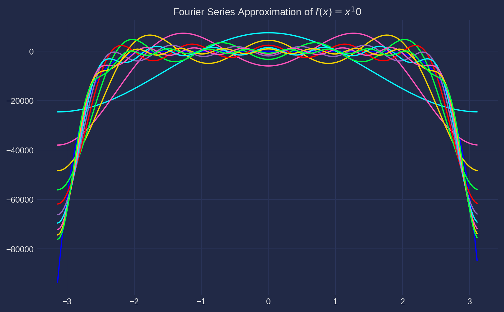
Gibbs Phenomenon
dx = 0.01
x = np.pi * np.arange(-1, 1, dx)
n = 20  # Number of terms
f = np.sign(x)  # Target function

a0 = np.sum(f) * dx

a = np.zeros(n)
b = np.zeros(n)

fourier_series = a0 / 2

plt.figure(figsize=(10, 6))

plt.plot(x, f, label=r'Target function $f(x) = \operatorname{sign}(x)$', color='blue')

for i in range(n):
    a[i] = np.sum(f * np.cos((i + 1) * x)) * dx
    b[i] = np.sum(f * np.sin((i + 1) * x)) * dx
    fourier_series += a[i] * np.cos((i + 1) * x) + b[i] * np.sin((i + 1) * x)

    plt.plot(x, fourier_series, label=f'Fourier Series with {i+1} terms')

plt.title(r'Fourier Series Approximation of $f(x) = \operatorname{sign}(x)$')
plt.grid(True)


plt.show()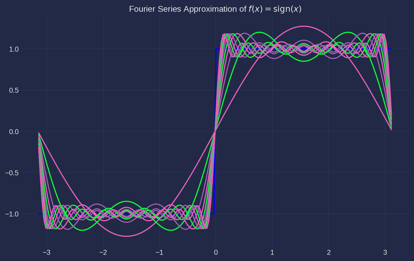
Complex Plane
Cartesian and Polar are two ways of representing complex numbers. In Cartesian form, a complex number is represented as a point in the complex plane. In Polar form, a complex number is represented by its magnitude and argument. \[ z = a + bi = r(\cos(\theta) + i\sin(\theta)) \]
Euler’s Formula
Euler’s formula is a mathematical formula that establishes the relationship between the trigonometric functions and the complex exponential function. It states that for any real number \(\theta\): \[ e^{i\theta} = \cos(\theta) + i\sin(\theta) \] Before I show you why this formula is true, let me show something more funmamental. The MacLaurin series of \(e^x\) is: \[ e^x = 1 + x + \frac{x^2}{2!} + \frac{x^3}{3!} + \frac{x^4}{4!} + \cdots = \sum_{n=0}^{\infty} \frac{x^n}{n!} \] If we plug in \(ix\) into the Taylor series, we get: \[ e^{ix} = 1 + ix + \frac{(ix)^2}{2!} + \frac{(ix)^3}{3!} + \frac{(ix)^4}{4!} + \cdots = 1 + ix - \frac{x^2}{2!} - i\frac{x^3}{3!} + \frac{x^4}{4!} + \cdots \] Note that even powers of \(x\) are real numbers and odd powers of \(x\) are imaginary numbers. If we separate the real and imaginary parts, we get: \[ e^{ix} = \underbrace{(1 - \frac{x^2}{2!} + \frac{x^4}{4!} - \cdots)}_{\cos(x)} + i\underbrace{(x - \frac{x^3}{3!} + \frac{x^5}{5!} - \cdots)}_{\sin(x)} = \cos(x) + i\sin(x) \] We used the facts of MacLaurin expansion of \(\cos(x)\) and \(\sin(x)\) to prove Euler’s formula.
Complex Fourier Series
To transform the Fourier series from the form expressed as a sum of sines and cosines:
\[ f(t)=a_0+\sum_{n=1}^{\infty} a_n \cos \left(\omega_n t\right)+b_n \sin \left(\omega_n t\right) \]
into the complex exponential form:
\[ f(t)=\sum_{n=-\infty}^{\infty} c_n e^{i \omega_n t} \]
we use Euler’s formulas for expressing sine and cosine in terms of exponentials:
\[ \begin{aligned} & \cos \left(\omega_n t\right)=\frac{e^{i \omega_n t}+e^{-i \omega_n t}}{2} \\ & \sin \left(\omega_n t\right)=\frac{e^{i \omega_n t}-e^{-i \omega_n t}}{2 i} \end{aligned} \]
Substitute these into the Fourier series: \[ \begin{aligned} f(t)&=a_0+\sum_{n=1}^{\infty} a_n\left(\frac{e^{i \omega_n t}+e^{-i \omega_n t}}{2}\right)+b_n\left(\frac{e^{i \omega_n t}-e^{-i \omega_n t}}{2 i}\right) &= a_0+\sum_{n=1}^{\infty} \frac{a_n-i b_n}{2} e^{i \omega_n t}+\sum_{n=1}^{\infty} \frac{a_n+i b_n}{2} e^{-i \omega_n t} \end{aligned} \]
Define the complex Fourier coefficients \(c_n\) and \(c_{-n}\): \[ \begin{aligned} c_n&=\frac{a_n-i b_n}{2} \\ c_{-n}&=\frac{a_n+i b_n}{2} \end{aligned} c_0 = a_0 \] Then the Fourier series can be expressed as: \[ f(t)=\sum_{n=-\infty}^{\infty} c_n e^{i \omega_n t} \]